
Sorting algorithms are a fundamental part of computer science and have a variety of applications, ranging from sorting data in databases to organizing music playlists. But what exactly are sorting algorithms, and how do they work? We’ll answer that question in this article by providing a comprehensive look at the different types algorithms and their uses, including sample code.
Essentially, a sorting algorithm is a computer program that organizes data into a specific order, such as alphabetical order or numerical order, usually either ascending or descending.
Sorting algorithms are mainly used to rearrange large amounts of data in an efficient manner so that it can be searched and manipulated more easily. They are also used to improve the efficiency of other algorithms such as searching and merging, which rely on sorted data for their operations.
There are various types of sorting available. The choice of sorting algorithm depends on various factors, such as the size of the data set, the type of data being sorted, and the desired time and space complexity.
These compare elements of the data set and determine their order based on the result of the comparison. Examples of comparison-based sorting algorithms include bubble sort, insertion sort, quicksort, merge sort, and heap sort.
These don’t compare elements directly, but rather use other properties of the data set to determine their order. Examples of non-comparison-based sorting algorithms include counting sort, radix sort, and bucket sort.
These algorithms sort the data set in-place, meaning they don’t require additional memory to store intermediate results. Examples of in-place sorting algorithms include bubble sort, insertion sort, quicksort, and shell sort.
These preserve the relative order of equal elements in the data set. Examples of stable sorting algorithms include insertion sort, merge sort, and Timsort.
These take advantage of any existing order in the data set to improve their efficiency. Examples of adaptive sorting algorithms include insertion sort, bubble sort, and Timsort.
Bubble sort is a simple sorting algorithm that repeatedly steps through a given list of items, comparing each pair of adjacent items and swapping them if they’re in the wrong order. The algorithm continues until it makes a pass through the entire list without swapping any items. Bubble sort is also sometimes referred to as “sinking sort”.
The origins of bubble sort trace back to the late 1950s, with Donald Knuth popularizing it in his classic 1968 book The Art of Computer Programming. Since then, it’s been widely used in various applications, including sorting algorithms for compilers, sorting elements in databases, and even in the sorting of playing cards.
Bubble sort is considered to be a relatively inefficient sorting algorithm, as its average and worst-case complexity are both $O(n^2)$ . This makes it much less efficient than most other sorting algorithms, such as quicksort or mergesort. Technical Note: $O(n^2)$ complexity means that the time it takes for an algorithm to finish is proportional to the square of the size of the input. This means that larger input sizes cause the algorithm to take significantly longer to complete. For example, if you consider an algorithm that sorts an array of numbers, it may take one second to sort an array of ten numbers, but it could take four seconds to sort an array of 20 numbers. This is because the algorithm must compare each element in the array with every other element, so it must do 20 comparisons for the larger array, compared to just ten for the smaller array. It is, however, very simple to understand and implement, and it’s often used as an introduction to sort and as a building block for more complex algorithms. But these days it’s rarely used in practice.
def bubble_sort(items): for i in range(len(items)): for j in range(len(items)-1-i): if items[j] > items[j+1]: items[j], items[j+1] = items[j+1], items[j] return items items = [6,20,8,19,56,23,87,41,49,53] print(bubble_sort(items)) function bubbleSort(items) let swapped; do swapped = false; for (let i = 0; i items.length - 1; i++) if (items[i] > items[i + 1]) let temp = items[i]; items[i] = items[i + 1]; items[i + 1] = temp; swapped = true; > > > while (swapped); return items; > let items = [6, 20, 8, 19, 56, 23, 87, 41, 49, 53]; console.log(bubbleSort(items)); Insertion sort is another simple algorithm that builds the final sorted array one item at a time, and it’s named like this for the way smaller elements are inserted into their correct positions in the sorted array.
In The Art of Computer Programming, Knuth comments that insertion sort “was mentioned by John Mauchly as early as 1946, in the first published discussion of computer sorting”, describing it as a “natural” algorithm that can easily be understood and implemented. By the late 1950s, Donald L. Shell made series of improvements in his shell sort method (covered below), which compares elements separated by a distance that decreases on each pass, reducing the algorithm’s complexity to $O(n^)$ and $O(n^)$ in two different variants. This might not sound as much, but it’s quite a significant improvement for practical applications! Technical Notes: $O(n^)$ and $O(n^)$ complexities are more efficient than $O(n^2)$ complexity, meaning they take less time to finish. This is because they don’t need to perform as many comparisons as $O(n^2)$ complexity. For example, it may take one second to sort an array of ten numbers using a $O(n^2)$ algorithm, but it could take 0.5 seconds to sort the same array using a $O(n^)$ algorithm. This is because the algorithm can perform fewer comparisons when using the $O(n^)$ algorithm, resulting in a faster runtime. In 2006 Bender, Martin Farach-Colton, and Mosteiro published a new variant of insertion sort called library sort or “gapped insertion sort”, which leaves a small number of unused spaces (or “gaps”) spread throughout the array, further improving the running time to $O(n \log n)$ . Technical Notes: $O(n \log n)$ complexity is more efficient than $O(n^2)$ complexity, and $O(n^)$ and $O(n^)$ complexities. This is because it uses a divide-and-conquer approach, which means that it can break the problem into smaller pieces and solve them more quickly. For example, it may take one second to sort an array of ten numbers using a $O(n^2)$ algorithm, 0.5 seconds to sort the same array using a $O(n^)$ algorithm, but it could take 0.1 seconds to sort the same array using a $O(n \log n)$ algorithm. This is because the algorithm can break the array into smaller pieces and solve them in parallel, resulting in a faster runtime.
Insertion sort is often used in practice for small data sets or as a building block for more complex algorithms. Just like with bubble sort, its worst-case and average-case time complexity is $O(n^2)$ . But unlike bubble sort, insertion sort can be used to sort data sets in-place, meaning that it doesn’t require additional memory to store intermediate results.
def insertion_sort(items): for i in range(1, len(items)): j = i while j > 0 and items[j-1] > items[j]: items[j-1], items[j] = items[j], items[j-1] j -= 1 return items items = [6,20,8,19,56,23,87,41,49,53] print(insertion_sort(items)) function insertionSort(items) for (let i = 1; i items.length; i++) let j = i; while (j > 0 && items[j - 1] > items[j]) let temp = items[j]; items[j] = items[j - 1]; items[j - 1] = temp; j--; > > return items; > let items = [6, 20, 8, 19, 56, 23, 87, 41, 49, 53]; console.log(insertionSort(items)); Quicksort is a popular divide-and-conquer sorting algorithm based on the principle of partitioning an array into two sub-arrays — one containing elements smaller than a “pivot” element and the other containing elements larger than the pivot element. The two sub-arrays are then sorted recursively. The basic steps of quicksort include:
Quicksort was invented by Tony Hoare in 1959. Hoare was working at the Elliott Brothers computer company in Britain when he developed the algorithm as a way to sort words in the memory of the Ferranti Mark I computer
. Quicksort was initially published as a research paper in 1961, and it quickly became one of the most widely used sorting algorithms due to its simplicity, efficiency, and ease of implementation.
Its worst-case time complexity is $O(n^2)$ when the pivot is chosen poorly, making it less efficient than other algorithms like merge sort or heapsort in certain situations. Technical Note: we don’t want to choose a pivot that’s too small or too big, or the algorithm will run in quadratic time. The ideal would be to choose the median as the pivot, but it’s not always possible unless we have prior knowledge of the data distribution.
def quick_sort(items): if len(items) > 1: pivot = items[0] left = [i for i in items[1:] if i pivot] right = [i for i in items[1:] if i >= pivot] return quick_sort(left) + [pivot] + quick_sort(right) else: return items items = [6,20,8,19,56,23,87,41,49,53] print(quick_sort(items)) function quickSort(items) if (items.length > 1) let pivot = items[0]; let left = []; let right = []; for (let i = 1; i items.length; i++) if (items[i] pivot) left.push(items[i]); > else right.push(items[i]); > > return quickSort(left).concat(pivot, quickSort(right)); > else return items; > > let items = [6, 20, 8, 19, 56, 23, 87, 41, 49, 53]; console.log(quickSort(items)); 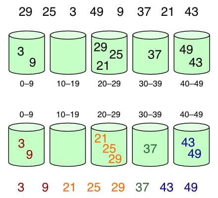
Bucket sort is a useful algorithm for sorting uniformly distributed data, and it can easily be parallelized for improved performance. The basic steps of bucket sort include:
Bucket sort is less efficient than other sorting algorithms on data that isn’t uniformly distributed, with a worst-case performance of $O(n^2)$ . Additionally, it requires additional memory to store the buckets, which can be a problem for very large data sets.
The are implementations of bucket sort already in the 1950s, with sources claiming the method has been around since the 1940s. Either way, it’s still in widespread use these days.
def bucket_sort(items): buckets = [[] for _ in range(len(items))] for item in items: bucket = int(item/len(items)) buckets[bucket].append(item) for bucket in buckets: bucket.sort() return [item for bucket in buckets for item in bucket] items = [6,20,8,19,56,23,87,41,49,53] print(bucket_sort(items)) function bucketSort(items) let buckets = new Array(items.length); for (let i = 0; i buckets.length; i++) buckets[i] = []; > for (let j = 0; j items.length; j++) let bucket = Math.floor(items[j] / items.length); buckets[bucket].push(items[j]); > for (let k = 0; k buckets.length; k++) buckets[k].sort(); > return [].concat(. buckets); > let items = [6, 20, 8, 19, 56, 23, 87, 41, 49, 53]; console.log(bucketSort(items)); Shell sort uses an insertion sort algorithm, but instead of sorting the entire list at once, the list is divided into smaller sub-lists. These sub-lists are then sorted using an insertion sort algorithm, thus reducing the number of exchanges needed to sort the list. Also known as “Shell’s method”, it works by first defining a sequence of integers called the increment sequence. The increment sequence is used to determine the size of the sub-lists that will be sorted independently. The most commonly used increment sequence is “the Knuth sequence”, which is defined as follows (where $h$ is interval with initial value and $n$ is the length of the list):
h = 1 while h n: h = 3*h + 1 Once the increment sequence has been defined, the Shell sort algorithm proceeds by sorting the sub-lists of elements. The sub-lists are sorted using an insertion sort algorithm, with the increment sequence as the step size. The algorithm sorts the sub-lists, starting with the largest increment and then iterating down to the smallest increment. The algorithm stops when the increment size is 1 , at which point it’s equivalent to a regular insertion sort algorithm.
Shell sort was invented by Donald Shell in 1959 as a variation of insertion sort, which aims to improve its performance by breaking the original list into smaller sub-lists and sorting these sub-lists independently.
It can be difficult to predict the time complexity of shell sorting, as it depends on the choice of increment sequence.
def shell_sort(items): sublistcount = len(items)//2 while sublistcount > 0: for start in range(sublistcount): gap_insertion_sort(items, start, sublistcount) sublistcount = sublistcount // 2 return items def gap_insertion_sort(items, start, gap): for i in range(start+gap, len(items), gap): currentvalue = items[i] position = i while position >= gap and items[position-gap] > currentvalue: items[position] = items[position-gap] position = position-gap items[position] = currentvalue items = [6,20,8,19,56,23,87,41,49,53] print(shell_sort(items)) function shellSort(items) let sublistcount = Math.floor(items.length / 2); while (sublistcount > 0) for (let start = 0; start sublistcount; start++) gapInsertionSort(items, start, sublistcount); > sublistcount = Math.floor(sublistcount / 2); > return items; > function gapInsertionSort(items, start, gap) for (let i = start + gap; i items.length; i += gap) let currentValue = items[i]; let position = i; while (position >= gap && items[position - gap] > currentValue) items[position] = items[position - gap]; position = position - gap; > items[position] = currentValue; > > let items = [6, 20, 8, 19, 56, 23, 87, 41, 49, 53]; console.log(shellSort(items)); The basic idea of merge sort is to divide the input list in half, sort each half recursively using merge sort, and then merge the two sorted halves back together. The merge step is performed by repeatedly comparing the first element of each half and adding the smaller of the two to the sorted list. This process is repeated until all elements have been merged back together.
Merge sort has a time complexity of $O(n \log n)$ in the worst-case scenario, which makes it more efficient than other popular sorting algorithms such as bubble sort, insertion sort, or selection sort. Merge sort is also a algorithm, meaning that it preserves the relative order of equal elements.
Merge sort has some disadvantages when it comes to memory usage. The algorithm requires additional memory to store the two halves of the list during the divide step, as well as additional memory to store the final sorted list during the merge step. This can be a concern when sorting very large lists.
Merge sort was invented by John von Neumann in 1945, as a comparison-based sorting algorithm that works by dividing an input list into smaller sub-lists, sorting those sub-lists recursively, and then merging them back together to produce the final sorted list.
def merge_sort(items): if len(items) 1: return items mid = len(items) // 2 left = items[:mid] right = items[mid:] left = merge_sort(left) right = merge_sort(right) return merge(left, right) def merge(left, right): merged = [] left_index = 0 right_index = 0 while left_index len(left) and right_index len(right): if left[left_index] > right[right_index]: merged.append(right[right_index]) right_index += 1 else: merged.append(left[left_index]) left_index += 1 merged += left[left_index:] merged += right[right_index:] return merged items = [6,20,8,19,56,23,87,41,49,53] print(merge_sort(items)) function mergeSort(items) if (items.length 1) return items; > let mid = Math.floor(items.length / 2); let left = items.slice(0, mid); let right = items.slice(mid); return merge(mergeSort(left), mergeSort(right)); > function merge(left, right) let merged = []; let leftIndex = 0; let rightIndex = 0; while (leftIndex left.length && rightIndex right.length) if (left[leftIndex] > right[rightIndex]) merged.push(right[rightIndex]); rightIndex++; > else merged.push(left[leftIndex]); leftIndex++; > > return merged.concat(left.slice(leftIndex)).concat(right.slice(rightIndex)); > let items = [6, 20, 8, 19, 56, 23, 87, 41, 49, 53]; console.log(mergeSort(items)); repeatedly selects the smallest element from an unsorted portion of a list and swaps it with the first element of the unsorted portion. This process continues until the entire list is sorted.
Selection sort is a simple and intuitive sorting algorithm that’s been around since the early days of computer science. It’s likely that similar algorithms were developed independently by researchers in the 1950s. It was one of the first sorting algorithms to be developed, and it remains a popular algorithm for educational purposes and for simple sorting tasks.
Selection sort is used in some applications where simplicity and ease of implementation are more important than efficiency. It’s also useful as a teaching tool for introducing students to sorting algorithms and their properties, as it’s easy to understand and implement.
Despite its simplicity, selection sort is not very efficient compared to other sorting algorithms such as merge sort or quicksort. It has a worst-case time complexity of $O(n^2)$ , and it can take a long time to sort large lists. Selection sort also isn’t a stable sorting algorithm, meaning that it may not preserve the order of equal elements.
def selection_sort(items): for i in range(len(items)): min_idx = i for j in range(i+1, len(items)): if items[min_idx] > items[j]: min_idx = j items[i], items[min_idx] = items[min_idx], items[i] return items items = [6,20,8,19,56,23,87,41,49,53] print(selection_sort(items)) function selectionSort(items) let minIdx; for (let i = 0; i items.length; i++) minIdx = i; for (let j = i + 1; j items.length; j++) if (items[j] items[minIdx]) minIdx = j; > > let temp = items[i]; items[i] = items[minIdx]; items[minIdx] = temp; > return items; > let items = [6, 20, 8, 19, 56, 23, 87, 41, 49, 53]; console.log(selectionSort(items)); The basic idea behind radix sort is to sort data by grouping it by each digit in the numbers or characters being sorted, from right to left or left to right. This process is repeated for each digit, resulting in a sorted list. Its worst-case performance is $

Radix sort was first introduced by Herman Hollerith in the late 19th century as a way to efficiently sort data on punched cards, where each column represented a digit in the data. It was later adapted and popularized by several researchers in the mid-20th century to sort binary data by grouping the data by each bit in the binary representation. But it’s also used to sort string data, where each character is treated as a digit in the sort. In recent years, radix sort has seen renewed interest as a sorting algorithm for parallel and distributed computing environments, as it’s easily parallelizable and can be used to sort large data sets in a distributed fashion.
Radix sort is a linear-time sorting algorithm, meaning that its time complexity is proportional to the size of the input data. This makes it an efficient algorithm for sorting large data sets, although it may not be as efficient as other sorting algorithms for smaller data sets. Its linear-time complexity and stability make it a useful tool for sorting large data sets, and its parallelizability (yeah, that’s an actual word) makes it useful for sorting data in distributed computing environments. Radix sort is also a stable sorting algorithm, meaning that it preserves the relative order of equal elements.
def radix_sort(items): max_length = False tmp, placement = -1, 1 while not max_length: max_length = True buckets = [list() for _ in range(10)] for i in items: tmp = i // placement buckets[tmp % 10].append(i) if max_length and tmp > 0: max_length = False a = 0 for b in range(10): buck = buckets[b] for i in buck: items[a] = i a += 1 placement *= 10 return items items = [6,20,8,19,56,23,87,41,49,53] print(radix_sort(items)) function radixSort(items) let maxLength = false; let tmp = -1; let placement = 1; while (!maxLength) maxLength = true; let buckets = Array.from( length: 10 >, () => []); for (let i = 0; i items.length; i++) tmp = Math.floor(items[i] / placement); buckets[tmp % 10].push(items[i]); if (maxLength && tmp > 0) maxLength = false; > > let a = 0; for (let b = 0; b 10; b++) let buck = buckets[b]; for (let j = 0; j buck.length; j++) items[a] = buck[j]; a++; > > placement *= 10; > return items; > let items = [6, 20, 8, 19, 56, 23, 87, 41, 49, 53]; console.log(radixSort(items)); Comb sort compares pairs of elements that are a certain distance apart, and swap them if they’re out of order. The distance between the pairs is initially set to the size of the list being sorted, and is then reduced by a factor (called the “shrink factor”) with each pass, until it reaches a minimum value of $1$ . This process is repeated until the list is fully sorted. The comb sort algorithm is similar to the bubble sort algorithm, but with a larger gap between the compared elements. This larger gap allows for larger values to move more quickly to their correct position in the list.
The comb sort algorithm is a relatively recent sorting algorithm that was first introduced in 1980 by Włodzimierz Dobosiewicz and Artur Borowy. The algorithm was inspired by the idea of using a comb to straighten out tangled hair, and it uses a similar process to straighten out a list of unsorted values.
Comb sort has a worst-case time complexity of $O(n^2)$ , but in practice it’s often faster than other $O(n^2)$ sorting algorithms such as bubble sort, due to its use of the shrink factor. The shrink factor allows the algorithm to quickly move large values towards their correct position, reducing the number of passes required to fully sort the list.
def comb_sort(items): gap = len(items) shrink = 1.3 sorted = False while not sorted: gap //= shrink if gap 1: sorted = True else: for i in range(len(items)-gap): if items[i] > items[i+gap]: items[i],items[i+gap] = items[i+gap],items[i] return bubble_sort(items) def bubble_sort(items): for i in range(len(items)): for j in range(len(items)-1-i): if items[j] > items[j+1]: items[j], items[j+1] = items[j+1], items[j] return items items = [6,20,8,19,56,23,87,41,49,53] print(comb_sort(items)) function combSort(items) let gap = items.length; let shrink = 1.3; let sorted = false; while (!sorted) gap = Math.floor(gap / shrink); if (gap 1) sorted = true; > else for (let i = 0; i items.length - gap; i++) if (items[i] > items[i + gap]) let temp = items[i]; items[i] = items[i + gap]; items[i + gap] = temp; > > > > return bubbleSort(items); > function bubbleSort(items) let swapped; do swapped = false; for (let i = 0; i items.length - 1; i++) if (items[i] > items[i + 1]) let temp = items[i]; items[i] = items[i + 1]; items[i + 1] = temp; swapped = true; > > > while (swapped); return items; > let items = [6, 20, 8, 19, 56, 23, 87, 41, 49, 53]; console.log(combSort(items)); The Timsort algorithm works by dividing the input data into smaller sub-arrays, and then using insertion sort to sort these sub-arrays. These sorted sub-arrays are then combined using merge sort to produce a fully sorted array. Timsort has a worst-case time complexity of $O(n \log n)$ , which makes it efficient for sorting large data sets. It’s also a stable sorting algorithm, meaning that it preserves the relative order of equal elements.
One of the key features of Timsort is its ability to handle different types of data efficiently. It does this by detecting “runs”, which are sequences of elements that are already sorted. Timsort then combines these runs in a way that minimizes the number of comparisons and swaps required to produce a fully sorted array. Another important feature of Timsort is its ability to handle data that’s partially sorted. In this case, Timsort can detect the partially sorted regions and use insertion sort to quickly sort them, reducing the time required to fully sort the data.
Timsort was developed by Tim Peters in 2002 for use in the Python programming language. It’s a hybrid sorting algorithm that uses a combination of insertion sort and merge sort techniques, and is designed to efficiently sort a variety of different types of data. It’s since been adopted by several other programming languages, including Java and C#, due to its efficiency and versatility in handling different types of data.
def insertion_sort(arr, left=0, right=None): if right is None: right = len(arr) - 1 for i in range(left + 1, right + 1): key_item = arr[i] j = i - 1 while j >= left and arr[j] > key_item: arr[j + 1] = arr[j] j -= 1 arr[j + 1] = key_item return arr def merge(left, right): if not left: return right if not right: return left if left[0] right[0]: return [left[0]] + merge(left[1:], right) return [right[0]] + merge(left, right[1:]) def timsort(arr): min_run = 32 n = len(arr) for i in range(0, n, min_run): insertion_sort(arr, i, min((i + min_run - 1), n - 1)) size = min_run while size n: for start in range(0, n, size * 2): midpoint = start + size - 1 end = min((start + size * 2 - 1), (n-1)) merged_array = merge( left=arr[start:midpoint + 1], right=arr[midpoint + 1:end + 1] ) arr[start:start + len(merged_array)] = merged_array size *= 2 return arr items = [6,20,8,19,56,23,87,41,49,53] print(timsort(items)) function insertionSort(arr, left = 0, right = arr.length - 1) for (let i = left + 1; i right; i++) const keyItem = arr[i]; let j = i - 1; while (j >= left && arr[j] > keyItem) arr[j + 1] = arr[j]; j--; > arr[j + 1] = keyItem; > return arr; > function merge(left, right) let i = 0; let j = 0; const merged = []; while (i left.length && j right.length) if (left[i] right[j]) merged.push(left[i]); i++; > else merged.push(right[j]); j++; > > return merged.concat(left.slice(i)).concat(right.slice(j)); > function timsort(arr) const minRun = 32; const n = arr.length; for (let i = 0; i n; i += minRun) insertionSort(arr, i, Math.min(i + minRun - 1, n - 1)); > let size = minRun; while (size n) for (let start = 0; start n; start += size * 2) const midpoint = start + size - 1; const end = Math.min(start + size * 2 - 1, n - 1); const merged = merge( arr.slice(start, midpoint + 1), arr.slice(midpoint + 1, end + 1) ); arr.splice(start, merged.length, . merged); > size *= 2; > return arr; > let items = [6, 20, 8, 19, 56, 23, 87, 41, 49, 53]; console.log(timsort(items)); Note that the time complexity and space complexity listed in the table are worst-case complexities, and actual performance may vary depending on the specific implementation and input data.
| Algorithm | Time Complexity | Space Complexity | In-place Sorting | Stable Sorting | Adaptive Sorting |
|---|---|---|---|---|---|
| Bubble sort | $O(n^2)$ | $O(1)$ | Yes | Yes | No |
| Quicksort | $O(n \log n)$ | $O(\log n)$ | Yes | No | Yes |
| Bucket sort | $O(n+k)$ | $O(n+k)$ | No | Yes | No |
| Shell sort | $O(n \log n)$ | $O(1)$ | Yes | No | No |
| Merge sort | $O(n \log n)$ | $O(n)$ | No | Yes | No |
| Selection sort | $O(n^2)$ | $O(1)$ | Yes | No | No |
| Radix sort | $O(w \cdot n)$ | $O(w+n)$ | No | Yes | No |
| Comb sort | $O(n^2)$ | $O(1)$ | Yes | No | Yes |
| Timsort | $O(n \log n)$ | $O(n)$ | Yes | Yes | Yes |
The most commonly used sorting algorithm is probably quicksort. It’s widely used in many programming languages, including C, C++, Java, and Python, as well as in many software applications and libraries. Quicksort is favored for its efficiency and versatility in handling different types of data, and is often used as the default sorting algorithm in programming languages and software frameworks. However, other sorting algorithms like merge sort and Timsort are also commonly used in various applications due to their efficiency and unique features.
Knowing the basics of sorting algorithms is essential for anyone interested in programming, data analysis, or computer science. By understanding the different sorting algorithms and their characteristics, you can improve your ability to select and implement the best algorithm for your specific use case. The best choice of sorting algorithm depends on several factors, including the size of the input data, the distribution of the data, the available memory, and the desired time complexity. Sorting algorithms can be categorized based on their time complexity, space complexity, in-place sorting, stable sorting, and adaptive sorting. It’s important to understand the characteristics and trade-offs of different sorting algorithms to select the most appropriate algorithm for a specific use case.
The choice of sorting algorithm can significantly impact the efficiency of your program. Different algorithms have different time complexities, which determine how fast they can sort data. For instance, Quick Sort is generally faster than Bubble Sort for large data sets due to its lower time complexity. Therefore, understanding the strengths and weaknesses of each algorithm can help you choose the most efficient one for your specific use case.
Stability in sorting algorithms refers to the preservation of the relative order of equal sort items. Stable algorithms maintain the original sequence of equal elements, while unstable algorithms do not. This characteristic is crucial in certain applications. For example, in a list sorted by name, a stable sort by age would keep the names in order within each age group.
Internal sorting algorithms are used when the entire data set can fit into the main memory of the computer. Examples include Bubble Sort, Insertion Sort, and Quick Sort. On the other hand, external sorting algorithms are used for large data sets that cannot fit into the main memory. These algorithms involve dividing the data into smaller chunks, sorting them individually, and then merging them.
In Quick Sort, the pivot is an element used to partition the data set. The choice of pivot can significantly affect the algorithm’s efficiency. If the pivot is always the smallest or largest element, Quick Sort performs poorly with a time complexity of O(n^2). However, if the pivot is chosen such that it always divides the array into two equal halves, the time complexity improves to O(n log n).
Bubble Sort is often considered inefficient due to its high time complexity of O(n^2) for worst and average cases. This means that the time it takes to sort the data increases quadratically with the number of elements. Therefore, Bubble Sort is generally not suitable for large data sets.
Merge Sort is a stable sorting algorithm with a time complexity of O(n log n) for all cases, making it more efficient than algorithms like Bubble Sort and Insertion Sort for large data sets. It also works well with linked lists, as it requires only constant extra space for linked lists, unlike arrays.
Heap Sort works by first transforming the list into a max heap – a binary tree where the parent node is always larger than its child nodes. The largest element (the root of the heap) is then swapped with the last element, effectively placing it in its correct position. The heap property is restored, and the process is repeated until the entire list is sorted.
Recursion is a method where the solution to a problem depends on solutions to smaller instances of the same problem. It is used in several sorting algorithms, including Quick Sort, Merge Sort, and Heap Sort. These algorithms divide the problem into smaller parts, solve them recursively, and combine the solutions to solve the original problem.
Counting Sort achieves linear time complexity by counting the occurrence of each element in the input list. It then cumulatively adds these counts to determine the position of each element in the output list. However, Counting Sort is not a comparison-based sort and requires a range of input data to be known beforehand.
Radix Sort is a non-comparative sorting algorithm that sorts numbers digit by digit, starting from the least significant digit to the most significant. It uses Counting Sort as a subroutine. Radix Sort has a time complexity of O(nk), where n is the number of elements and k is the number of digits in the maximum number. It is efficient when the range of input data is significantly larger than the number of elements to be sorted.
Lucero del Alba
Lucero is a programmer and entrepreneur with a feel for Python, data science and DevOps. Raised in Buenos Aires, Argentina, he's a musician who loves languages (those you use to talk to people) and dancing.